
2010 Volume Issue 2
December 2, 2010
For a downloadable version, click the following:
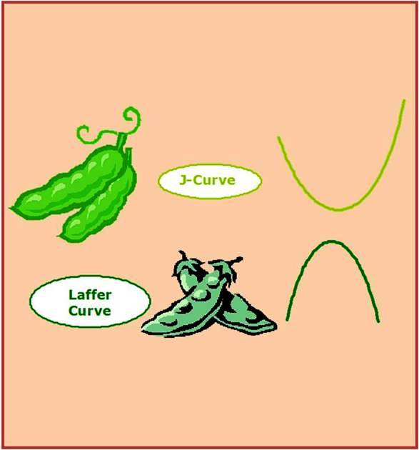
The Laffer Curve and the J-Curve are Analytically like Two Peas in a Pod
Economics is saturated with concepts, each having a large number of applications. One such concept is that of elasticity. This issue of the New Economic Paradigm Newsletter is about two such applications of elasticity; the J-Curve focuses on the effectiveness of exchange rate policies and the Trade and Current Account imbalances and the Laffer curve is about the efficacy of fiscal policies involving tax rate changes.
Elasticity measures the response of one variable to the change in another variable. In the news of late, two such elasticity relationships, the J-Curve and the Laffer curve have once again made the headlines.
THE J-CURVE AND INTERNATIONAL TRADE POLICY
We begin with an analysis of the J-Curve and its implications for a nation’s international trade and foreign exchange policy. The reason for the name, J-Curve, is that the letter J is a graphical picture of the relationship between a change in an exchange rate and the amount of a nation’s net foreign exchange earnings over time in response to this change in its exchange rate(s) with the currency of another nation(s).
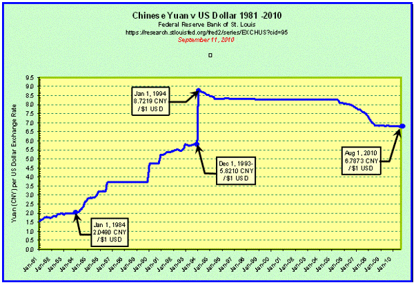
An example would be the U.S. Dollar price of a Chinese Yuan changing from $0.12 for 1 (¥) Yuan to $0.15 for 1 (¥) Yuan. This would also be termed a depreciation of the Dollar which can also be called an appreciation of the Yuan since these two exchange rates are reciprocals of each other.
In many cases, shortly after a currency is depreciated, as in the example just mentioned, the total resulting net earnings of foreign currency (Chinese Yuan) often decrease, then bottom out, and finally begin to rise resulting in a J shape in terms of the resulting Trade and Current Account Balances and in net foreign exchange earnings. But it takes the passage of time for this response to occur. For policy purposes, how long a time for the desired change to occur, is too long?
In the Balance of Payments Accounts (BOPA) terminology, the Trade Balance (same as the Balance on Merchandise and Services Accounts) could be used as the litmus test of the success or failure of a policy. The Current Account Balance, which consolidates the Trade Balance with the Unilateral Transfer Account Balance, is often used as alternative to judge the effects of the policy. Either way, it takes time for the effects of the depreciation of the dollar to increase the total net earnings of Chinese Yuan. The J-Curve is a picture of an elasticity relationship as explained below.
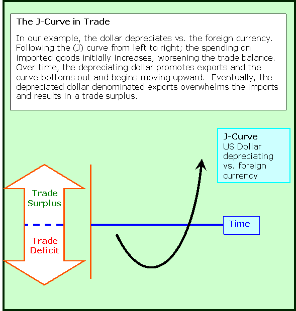
To reiterate, elasticity measures the response of one variable to the change in another. Response takes time and usually increases in a cumulative manner as time passes. Graphically, the foreign exchange earnings line will initially slope downward as foreign exchange earnings decrease. As time passes, the foreign exchange earnings line begins to flatten out and then rise reflecting a decreasing Trade balance deficit and perhaps even a Trade Balance surplus will develop. When this occurs, the foreign exchange earnings line rises above the X axis and the J-Curve is complete.
When the U.K. was experiencing large and persistent deficits in its Trade Balance in the Post WWII era, even as a member of the fixed exchange rate system often referred to as the Breton Woods IMF Fixed Exchange Rate System, they were allowed to devalue the British Pound (equivalent to depreciating the Pound in a floating exchange rate system) on a few occasions. Net foreign exchange earnings initially fell, as the Pound value of their trade deficit increased. However, in the parlance of J-Curve literature, the downward sloping first part of the J-Curve did not seem to bottom out and did not begin to rise, at least during the time period before the patience of the policy makers ran out.
A sophisticated argument commenced in which some highly regarded economists, such as Roy Harrod, asked whether the Pound should be revalued upward rather than devalued.
homepage.newschool.edu/het//profiles/harrod.htm
Roy F. Harrod, 1953 (The Dollar)
www.economyprofessor.com/theorists/royharrod.php
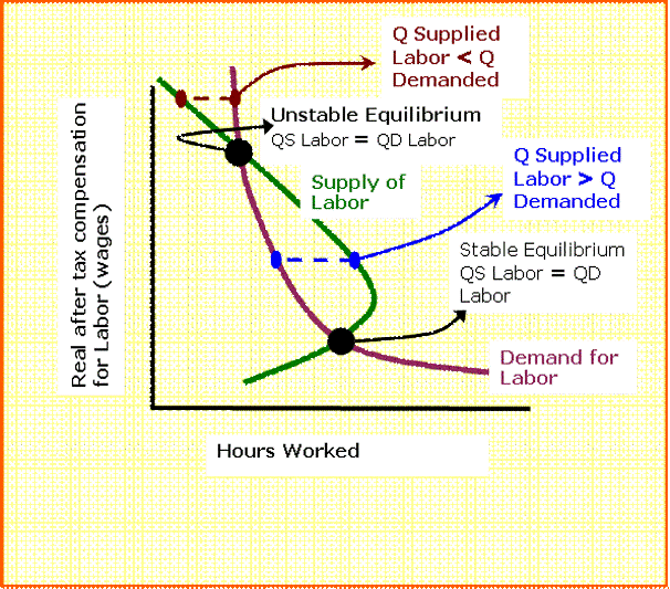
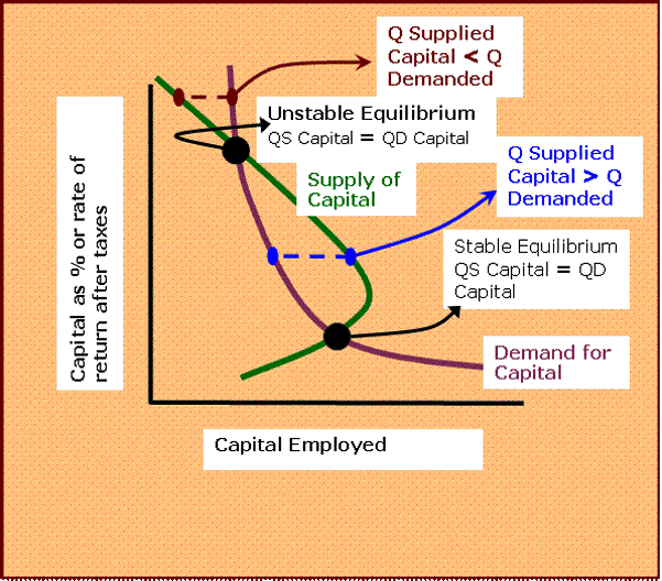
The argument revolved around the issue of whether the then current exchange rate was above an unstable equilibrium. In this range, due to a backward bending supply curve for foreign exchange, a price increase for the dollar (due to devaluing the Pound which means increasing the Pound price of the Dollar) would increase the shortage of Dollars, not decrease that shortage.
Some argued that the British pound should be revalued upward and not devalued.
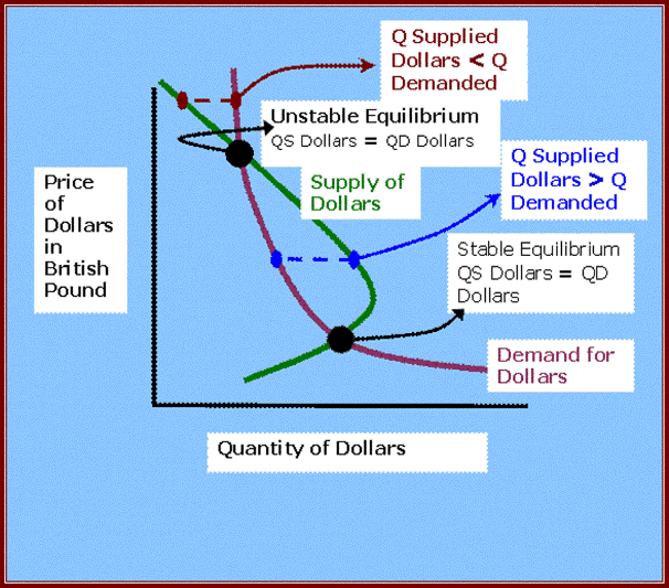
Was it just a question of time in order to let the response have its full effect? In other words, was it truly a J-Curve not given enough response time or was it a situation in which the relevant exchange rate was in the negatively sloped portion of a backward bending supply curve for foreign exchange and the passage of time would not show an improvement in the worsening Trade deficit?
Elasticities (Price Elasticity of Demand)
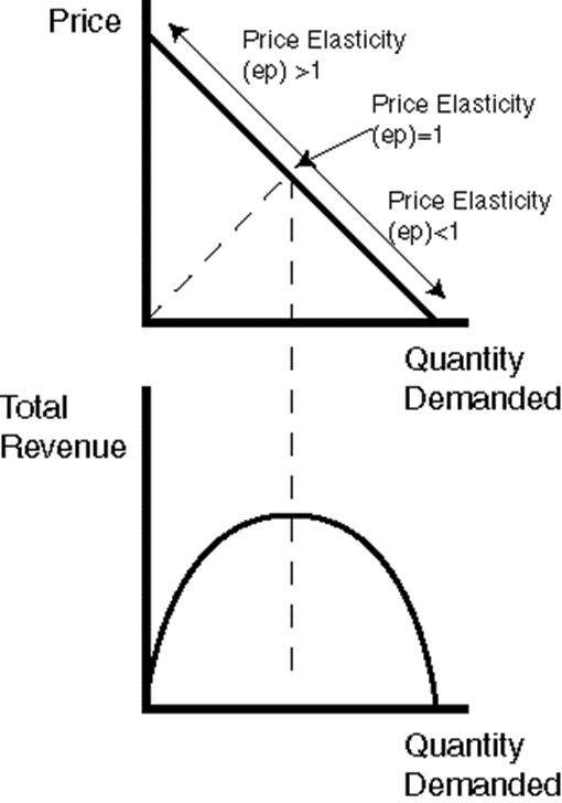
Let us first apply the analysis the crude oil market. If the price is cut in the range below the midpoint of the demand curve diagonal (remember at midpoint Ep=1, where Ep stands for the coefficient of price elasticity of demand) total revenue falls. It follows that total revenue expended on oil is maximized if the price charged corresponds to that where Ep=1.
This is not necessarily the case. The literature of international finance abounds with discussions of the Marshall-Lerner conditions that indicate that the equilibrium in the foreign exchange markets could be an unstable one. A rise in the price of foreign exchange could increase the current account deficit (surplus of domestic currency in foreign exchange market which is equivalent to a shortage of foreign exchange). Similarly, a fall in the price of foreign exchange could increase the surplus of foreign exchange or its equivalent, a shortage of the domestic currency. In other words, a depreciation of the domestic currency against foreign exchange could increase a trade account deficit; appreciation of the domestic currency against foreign exchange could increase the trade surplus depending on the range in which the change in the exchange rate occurs.
To understand why this is so, let us examine the market for crude oil in using the models in the Elasticity Graphic. We will assume a straight-line demand curve for oil to keep the discussion simple. Even most curvilinear demand curves, more or less, would be consistent with the following discussion. The mid-point of a straight line demand curve along the diagonal has a price elasticity of 1. In the range below the price where Ep = 1 (i.e. below the mid-point), the price elasticity is less than one, and it approaches zero the farther down the demand curve we move. Above the price corresponding to the mid-point of the demand curve diagonal, the Ep is greater than one. Recall from micro theory that if price is raised in the elastic range where Ep is greater than one, then total revenue expended on oil decreases. If the price is cut in the range below the midpoint of the demand curve diagonal (remember at midpoint Ep = 1) total revenue falls. It follows that total revenue expended on oil is maximized if the price charged corresponds to that where Ep = 1. This is not necessarily the point of profit maximization (unless costs are insignificant) but the point of revenue maximization. Thus in Figure 8.3, note that total revenue is maximized at the price, quantity combination where Ep = 1.
The relationship between a fall in the price of oil and the total revenue or expenditures on oil first rise, then reach a maximum, and then fall as price continuously falls. If OPEC was dominated by low cost producers (as it is), prices that maximize revenue or expenditures on oil, would not be too far from the price that maximized total profits.
When we examine the Laffer curve below, a similar confusion occurred concerning the behavior of total tax revenues in response to a tax rate cut and gave rise to a controversy similar to that surrounding the efficacy of the J-Curve argument that continues to this day.
Because of the persistent trade deficit with China, there has been an increasing cry for a depreciation of the dollar.
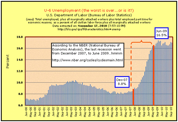
The problem has been exacerbated because of the high rate of unemployment in the U.S. measured by the U 3 definition it is at 9.6% of the labor force but by the more meaningful U 6 measure, the unemployment rate is 17.1%.
Trade deficits depress the economy. This is because imports depress and exports stimulate the level of economic activity. A trade deficit occurs when a nation’s imports exceed its exports. It is not only vis-à-vis mainland China with which the U.S. has Balance of Trade deficit, but it has very large and persistent deficits with many nations including those that are part of the European Union.
In an earlier issue of the Newsletter, an in depth analysis was presented which explained why and when this Trade Balance deficit with China began and why it has persisted for more than twenty years.
2010 Volume Issue 1
September 23, 2010
HERE WE GO AGAIN
The broken CD (record) routine…before it was Japan and Germany eating our lunch, now it is China
www.econnewsletter.com/sep232010
The short term results are often at odds with the longer run results of this intervention in the foreign exchange markets. In the U.S., such intervention in foreign exchange markets is usually carried out by the Federal Reserve System, our central bank.
A recent article by Robert Reich on the efficacy of a nation depreciating its currency in the Foreign Exchange Market reflects this confusion. This direction of results is more often due to the time period in which those results are measured, rather than a more fundamental problem such as a backward bending curve. Professor Reich’s article does not consider the historical context of this specific exchange rate policy, but is concerned about setting off a war of competitive depreciation of nation’s currencies.
Why It’s Foolish to Weaken the Dollar to Create Jobs
www.huffingtonpost.com/robert-reich/post.html
The argument for depreciating a nation’s currency in foreign exchange markets by intervention (termed devaluation in a fixed exchange rate system and depreciation in a floating rate system), is as follows. Trade deficits occur when the value of a nation’s imports exceed the value of its exports. Imports are a leakage or withdrawal and as such, depress a nation’s aggregate demand and hence the level of its economic activity and probably its employment level. Exports have the opposite effects. So by reducing a nation‘s trade deficit (a condition in which the value of its imports exceed the value of its exports (with China in our example), it reduces that depressant and thus stimulates that nation’s level of economic activity and probably reduces its unemployment rate. This assumes that the other nation does not retaliate since our depreciating the Dollar does have just the opposite effects on the other nation, in this case, China. It would tend to depress their level of economic activity and probably increase their unemployment rate. This is why such a U.S. policy increases the probability of China’s retaliation by depreciating the Yuan. Such retaliation was characteristic of the rounds of competitive depreciation of nation’s currencies that was common in the Great Depression of the 1930s.
What the U.S. policymakers would be doing is selling Dollars making them less scarce and buying Yuan making them scarcer. In this market, the demand curve for Yuan increases (the demand curve shifts upward and to the right or away from the origin) and thus causes the Dollar price of the Yuan to rise. The higher dollar price of the Yuan is termed a depreciation of the Dollar.
Remember that China has been intervening for nearly twenty years to depreciate the Yuan in respect to the Dollar from $0.50 to around $0.125 and then pegging or maintaining it there by continued intervention. (Again, for an in depth analysis of this issue, see our previous newsletter on this website which was posted several weeks ago.) Recently, the Chinese have relented slightly and allowed the Dollar price of the Yuan to rise to nearly $0.15 for 1 Yuan. The Dollar price of the Chinese Yuan is still very much below its equilibrium level.
The initial or short-term result may be an increase in the Dollar amount spent on U.S. imports from China and an initial increase in the Dollar value of U.S. Trade deficit. The short-term effect of this intervention appears to show that this policy has failed to achieve its objective of reducing that dollar value of the trade deficit. Recall that this is to be expected if the J-Curve argument is valid. But the response to the effectively higher price of imports from China (since the cost of the foreign currency or Yuan increased) will take time. As U.S. importers consider the effect of the Dollar depreciation on their costs and profits, they begin to look for alternative sources that are less expensive. As American importers shift to non-China sources including domestic U.S- sources, the trade deficit with China decreases as does the supply of Dollars to China.
As time passes, if the Chinese exporters do not cut the Yuan price of their goods and services, the quantity response by the U.S. importers should begin to increase significantly in a negative direction. Remember that in international transactions, two prices are involved, the Yuan price of Chinese goods and services and the Dollar price of the Yuan. The effective price of imports from China has increased due to the depreciation of the U.S. Dollar and thus a higher effective price for China’s goods and services to U.S. importers. The greater the substitution effect, the greater the decrease in the quantity demanded of imports of goods and services from China in response to an increase in the effective price of these imports of goods and services. U.S. importers may begin substituting other sources of goods and services for the Chinese ones.
History shows that if many of the past such similar episodes are the rule, the U.S. Trade Balance with China would then slow its increase and could eventually begin a decrease as Dollar expenditures on Chinese goods and services begin to decrease. In the J-Curve graph, during an initial period of time, the trade deficit may increase but would be followed by a decreasing trade deficit. As pointed out in an earlier issue of this Newsletter, this may provide a stimulus to the U.S. economy, but it would increase economic and political instability in China. This would lessen the ability of China to neutralize its nuclear neighbors, Pakistan, India and maybe North Korea.
At issue is the so called J-Curve reflecting a nation’s trade deficit after it pursues a policy of depreciating its currency in foreign exchange markets. Remember that such a policy can be offset if the exporting nation retaliates by selling its currency and buying Dollars or by increasing subsidies on their exports. Remember, the Chinese started to depreciate the Yuan nearly twenty years ago. Once they had achieved an exchange rate at which they were comfortable, they pegged it there by continued intervention in the foreign exchange markets down to this day. Too many critics and supporters fail to place this issue in its historical geopolitical context.
Alternative policies of increasing tariffs on U.S. imports are more likely to provoke retaliation by from other nations by imposing countervailing tariffs. The Great Depression also experienced several rounds of tariff wars that saw the importing nations depreciating their currencies by intervention in foreign exchange markets. Such tactics were used in the 1930’s, about which the Reich article hints. Also recall the infamous Smoot Hawley tariff in the U .S. Many nations employed their own version of our Smoot Hawley tariff. If we were not encountering a significant and continuing dismal job picture at home, in all likelihood, the issue of trade deficits, especially with China, would not have raised so much concern.
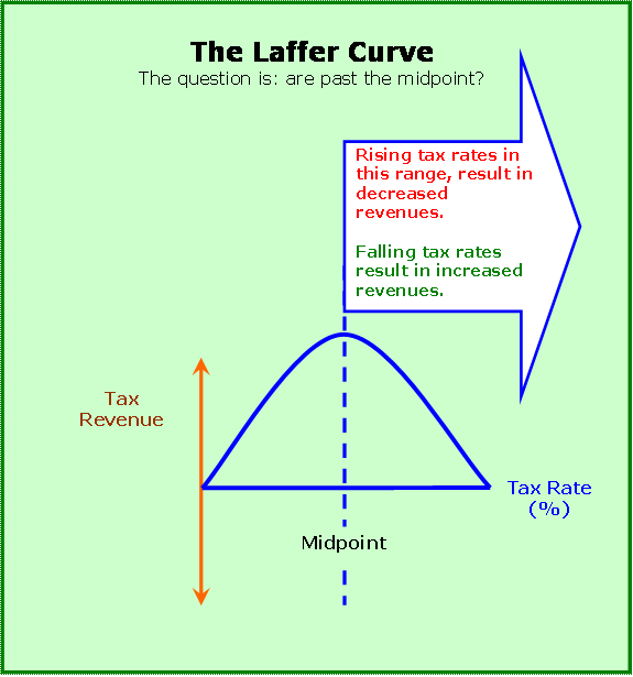
The Laffer Curve
While focusing on an entirely different topic, the argument posed by Arthur Laffer during the administration of Ronald Reagan is analytically similar to that of the J-Curve. In the case of the Laffer curve argument, the issue is, will a tax rate cut eventually cause a tax revenue increase and how long of a lag before the revenue increase occurs? Tax revenues are the product of the tax rate times the tax base. The tax in question is the income tax.
While it has been lumped in with the supply side literature, it is also a Keynesian argument. Taxes are a leakage or withdrawal and depress the level of economic activity by depressing aggregate demand due to the resulting lower Disposable (Personal) Income. Once again we are faced with an analysis that involves the response of one variable, tax revenues, to a change in another variable, the tax rate. The connection is that a tax rate cut stimulates the economy to a higher level of production and income and thus the tax base is increased. Tax revenues equal the tax base times the tax rate. This issue took front and center in the election of 2010 and will continue to remain at the forefront of debate for years to come.
In economic principles courses, students are taught that price elasticity of demand usually increases with the passage of time. In the very short run, a price decrease may not affect the quantity demanded of the good or service in question and may initially decrease total revenue. Human response takes time. However, as time passes, buyers will become responsive to the price decrease and buy more of the good or service in question (or less of the good or service in question if the price is increased).
The longer the time allowed for the measurement of the quantity response to a price change, usually the larger the change in quantity demanded. Similarly, a tax rate decrease may not immediately stimulate the level of economic activity and its accompanying rise in production and income and therefore in the very short run may not increase the tax base. But as time passes, while the cost of the productive resources to the employing firm does not change, the after tax reward to the productive resources increases and if the supply curve of these productive resources is sloping upward and to the right, a greater quantity supplied of these resources will result. This is true of all productive resources, including debt and equity capital as well as labor.
This is the basis of the supply-sider’s argument. The anti supply-siders implicitly argue that the supply curve of the productive resources has at least turned vertical and probably is bending backward (sloping upward and to the left, in the range of the before and after tax cut compensation rates. Interest rates for the suppliers of debt capital, total yield rates for the suppliers of equity capital and wage plus non-wage compensation rates for labor are among such rewards for productive resources. The correct economics term for such rewards is income. (The reader may find it helpful to go back to the earlier portion of this issue of the Newsletter and review the material on the backward bending supply of foreign exchange curve.)
(After this section on the Laffer curve, we will examine the theory of the concept of price elasticity of demand and its relation to the time period and the behavior of the total dollar response.)
Not unlike the argument behind J-Curve examined above, is the behavior of tax revenues responding to a cut in the tax rates. It is a two way relationship in that there is also an argument that a tax rate increase can eventually cause a decline in the tax base (GDP) and a decrease in tax revenues. The Rubinomics in the latter Clinton presidential years is cited as one such example. The collapse in the first quarter of 2000 was a major cause of the recession-like period greeting George Bush II as he began his presidential years.
Congressional Budget Office
As stated before, response to a change in a causal variable takes time. A crucial question in policy making is the length of time of the lags involved. Lengthy lags call into question the validity of the argument and the practicality of the policy even if the relationship is valid. Given enough time, the problem generating the policy, may change considerably. All recession turn into recoveries and all periods of significant growth, turn into slower growth and sometimes a recession.
THE THEORY OF PRICE ELASTICITY OF DEMAND
The “Law of Demand” refers to the market behavior of buyers. In almost all cases, as the price of a good or service such as college credit hours or ground beef decreases, the quantity demanded for that good or service, increases, as a result of that price decrease, all else equal. As the price of a good or service such as college tuition per credit hour or a pound of ground beef increases, the quantity demanded of credit hours or ground beef, decreases. Graphically, that is why nearly all demand curves for goods and services slope downward and to the right, reflecting the Law of Demand.
Similarly, if the supply of productive resources such as labor and capital are sloping upward and to the right in their upper regions of rewards per unit of resource as supply-siders implicitly argue, increases in after tax real compensation rates for labor and real after tax rates of return for debt and equity capital, result in a GREATER quantity supplied of each and not smaller as anti supply-siders implicitly argue. The quantity response will typically be greater – the longer the time period allowed to measure the response.
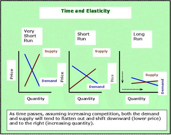
How much quantity demanded increases or decreases as a result of a price change, depends upon the time allowed to measure the quantity response of buyers as well as the strength of the soon to be described substation and income effects.
Since total revenue received by sellers in response to the price change is the price times the quantity demanded, the resulting change in total revenue depends upon the time allowed to measure the quantity response. The longer the time allowed for buyers and sellers to respond, most of the time the greater is the quantity response. Be careful not to jump to conclusions. A few decades ago, as the compensation to harvest labor began to rise in farming, farm implement manufacturers began to develop equipment to reduce the amount of labor needed to harvest crops. Agriculture scientists accelerated their efforts to develop crop varieties that could withstand the rougher treatment of mechanical harvesting equipment.
When some states passed minimum wage legislation and other benefits legislation for agricultural workers, when unions began to make inroads in this farm labor market, and when college age workers were shrinking in availability, a vast transformation began t occur in the technology of harvesting. In the area of the fruit industry for example, the development of dwarf tree varieties and more pliable materials that caught the fruit as mechanical shakers harvested the fruit, human workers were replaced with the productive resource, physical capital. Yes, this example of automation that not only occurs in manufacturing, but throughout the entire production process of both goods and services. This substitution effect in production is the equivalent of the substitution in consumption. The greater the substitution effect, the greater t he quantity response to a price change whether it be the firm’s demand for productive resources such as labor or capital or the demand for a good or service by a consumer.
The early studies of affects of minimum wage legislation and unionization allowed little time for the response of growers to adjust to the higher labor costs. As a result the researchers often argued their research showed little effect of higher labor costs on the demand for harvest labor in areas such as peanuts. Longer term studies however, showed significantly different results as technological change occurred and was implemented and cultivation and harvesting became increasingly capital intensive and less labor intensive. In this case, the substitution effect of physical capital for labor was strengthened by technological advances.
Now we can apply this concept that response takes time and longer run results often show that conclusions based on short-term response data are often very misleading.
Will depreciation of the U.S. Dollar appreciably reduce our Trade Balance Deficits?
Will repealing, or letting the so called Bush tax rate cuts expire under sunset provisions, decrease or increase the huge federal deficits?
Would extending the Bush tax rate cuts and even legislating further tax rate cuts reduce the federal deficits?
The readers are encouraged to take the analysis presented in this issue of the New Economic Paradigm Newsletter and review the history of the episodes when the J-Curve and the Laffer curve were postulated.
Coming soon to this website:
Pricing college tuition
We will be posting to this website, a newsletter on the topic of “Pricing College Education”. We will point out that institution of higher education seem to be following the same path as the former and failing Big Three American firms in the U.S. automotive firms have taken. There are striking similarities between the two. College education is the new “sticker shock”.
Price elasticity of demand is a critical issue that seems to be ignored or not understood by college administrators and their boards of trustees. “Fooled once, shame on you; fooled twice, shame on me”.
